Conic Optimization on Julia
Here I will describe a bit about conic programming on Julia based on
Juan Pablo Vielma’s JuliaCon 2020 talk and
JuMP devs Tutorials. We will begin by defining what is a cone and how to model them on JuMP together with some simple examples, by the end we will solve an mixed - integer conic problem of avoiding obstacles by following a polynomial trajectory.
Why Conic Optimizacion?
- Linear- programming-like duality
- Faster and more stable algorithms
- Avoid non-differentiability issues, exploit primal-dual form, strong theory on barriers for interior point algorithms.
- Industry change in 2018:
- Knitro version 11.0 adds support for SOCP constraints.
- Mosek version 9.0 deprecates expression/function-based formulations and focuses on pure conic (linear, SOCP, rotated SOCP, SDP, exp & power)
Table of Contents
- What is a Cone?
- Conic Programming.
- Some type of Cones supported by JuMP and programming examples.
- Second Order - Cone
- Rotated Second Order - Cone
- Exponential Cone
- Positive Semidefinite Cone (PSD)
- Other Cones and Functions.
- Mixed Integer Conic example: Avoiding obstacles (Drone and Flappy bird)
- Continuous Conic programming on Julia?
What is a Cone?
A subset $C$ of a vector space $V$ is a cone if $\forall x \in C$ and positive scalars $\alpha$, the product $\alpha x \in C$.
A cone C is a convex cone if $\alpha x + \beta y \in C$, for any positive scalars $\alpha, \beta$, and any $x, y \in C$."
Conic Programming
Conic programming problems are convex optimization problems in which a convex function is minimized over the intersection of an affine subspace and a convex cone. An example of a conic-form minimization problems, in the primal form is:
\begin{equation} \min_{ x \in \mathbb{R}^n} a_0 ^\top x + b_0 \end{equation}
such that: $$A_i x + b_i \in \mathcal{C}_i \quad \text{for } i = 1 \dotso m$$
The corresponding dual problem is:
$$ \max_{y_1, \dotso , y_m} - \sum_{i = 1}^{m} b_i ^T y_i + b_0$$
such that: $$ a_0 - \sum_{i = 1}^{m} A_{i}^{T} y_{i} = 0 $$ $$ y_i \in \mathcal{C}_i^*$$
Where each $\mathcal{C}_i$ is a closed convex cone and $\mathcal{C}_i^*$ is its dual cone.
Some of the Types of Cones supported by JuMP
Second - Order Cone
The Second - Order Cone (or Lorentz Cone) of dimension $n$ is of the form:
$$ Q^n = \{ (t,x) \in \mathbb{R}^n: t \ge \lVert x \rVert_2 \} $$
A Second - Order Cone rotated by $\pi/4$ in the $(x_1,x_2)$ plane is called a Rotated Second- Order Cone. It is of the form:
$$ Q^n_r = \{ (t,u,x) \in \mathbb{R}^n: 2tu \ge \lVert x \rVert_2, t, u \ge 0 \} $$
These cones are represented in JuMP using MOI sets SecondOrderCone and RotatedSecondOrderCone
Example: Euclidean Projection on a hyperplane
For a given point $u_0$ and a set $K$, we refer to any point $u \in K$ which is closest to $u_0$ as a projection of $u_0$ on $K$. The projection of a point $u_0$ on a hyperplane $K = \{ u : p'\cdot u = q \}$ is given by:
$$ \begin{align}
& \min_{x \in \mathbb{R}^n} & \lVert u - u_0 \rVert \\
& \text{s.t. } & p'\cdot u = q
\end{align}$$
We can model the above problem as the following conic program:
$$ \begin{align}
& \min & t \\
& \text{s.t. } & p'\cdot u = q \\
& \quad & (t, u - u_0) \in Q^{n+1}
\end{align}$$
If we transform this to the form we saw above,
$$ \begin{align}
x & = (t,u)\\
a_0 & = e_1\\
b_0 & = 0\\
A_1 & =(0,p)\\
b_1 & = -q \\
C_1 & = \mathbb{R}\\
A_2 & = 1\\
b_2 &= -(0,u_0)\\
C_2 &= Q^{n+1}
\end{align}$$
Thus, we can obtain the dual problem as:
$$ \begin{align}
& \max & y_1 + (0,u_0)^\top y_2 \\
& \text{s.t. } & e_1 -(0,p)^\top y_1 - y_2 = 0 \\
& \quad & y_1 \in \mathbb{R}\\
& \quad & y_2 \in Q^{n+1}
\end{align}$$
Let’s model this in Julia.
First we need to load some packages JuMP is the modeling package, ECOS is a solver, LinearAlgebra and Random are just to get some linear algebra operations and a fix seed for reproducibility respectively.
using JuMP
using ECOS
using LinearAlgebra
using Random
Random.seed!(2020);
Lets get some random values for the problem’s input: $u_0$, $p$ and $q$
u0 = rand(10)
p = rand(10)
q = rand();
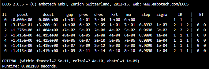
Now we can write the model:
model = Model(optimizer_with_attributes(ECOS.Optimizer, "printlevel" => 0))
@variable(model, u[1:10])
@variable(model, t)
@objective(model, Min, t)
@constraint(model, [t, (u - u0)...] in SecondOrderCone())
@constraint(model, u' * p == q)
optimize!(model)
Then we can see the objective function value and variable value at the optimum by doing:
@show objective_value(model);
@show value.(u);
We get an objective value of : $1.4149915748070703$. We can also solve the dual problem:
e1 = [1.0, zeros(10)...]
dual_model = Model(optimizer_with_attributes(ECOS.Optimizer, "printlevel" => 0))
@variable(dual_model, y1 <= 0.0)
@variable(dual_model, y2[1:11])
@objective(dual_model, Max, q * y1 + dot(vcat(0.0, u0), y2))
@constraint(dual_model, e1 - [0.0, p...] .* y1 - y2 .== 0.0)
@constraint(dual_model, y2 in SecondOrderCone())
optimize!(dual_model)
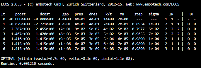
@show objective_value(dual_model);
We get an objective value of : $1.4149916455792486$. The difference between this value and the primal is $ \approx 7.07 \times 10^{-8}$, does this makes sense?
We can also have an equivalent formulation using a Rotated Second - Order cone:
$$ \begin{align}
& \min & t \\
& \text{s.t. } & p'\cdot u = q \\
& \quad & (t, 1/2, u - u_0) \in Q^{n+2}_r
\end{align}$$
model = Model(optimizer_with_attributes(ECOS.Optimizer, "printlevel" => 0))
@variable(model, u[1:10])
@variable(model, t)
@objective(model, Min, t)
@constraint(model, [t, 0.5, (u - u0)...] in RotatedSecondOrderCone())
@constraint(model, u' * p == q)
optimize!(model)
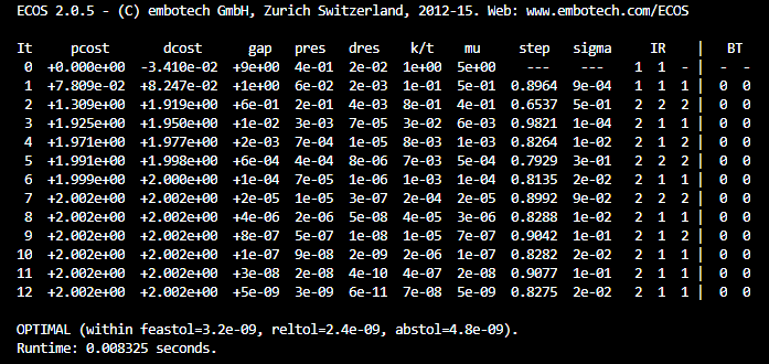
We notice that the objective function values are different. There is a simple explanation to that behaviour. In the case of Second-Order Cone the objective function is $\lVert u - u_0 \rVert _2$ while in the case of a Rotated Second-Order Cone is $\lVert u - u_0 \rVert_2^2$. However, the values of $u$ are the same in both problems.
Exponential Cone
An exponential Cone is a set of the form:
$$ K_{\exp} = \{ (x,y,z) \in \mathbb{R}^3 : y \cdot \exp(x/y) \le z, y \ge 0 \}$$
It is represented in JuMP using the MOI set ExponentialCone.
Example: Entropy Maximization
We want to maximize the entropy function $ H(x) = - x log (x)$ subject to linear inequality constraints.
$$ \begin{align}
& \max & -\sum_{i=1}^{n} x_ilog(x_i) \\
& \text{s.t. } & \mathbf{1}^\top x = 1\\
& \quad & Ax \le b
\end{align}$$
We just need to use the following transformation:
$$ t \le -xlog(x) \iff t \le x log(1/x) \iff (t,x,1) \in K_{\exp}$$
An example in Julia would be:
n = 15;
m = 10;
A = randn(m, n);
b = rand(m, 1);

model = Model(optimizer_with_attributes(ECOS.Optimizer, "printlevel" => 0))
@variable(model, t[1:n])
@variable(model, x[1:n])
@objective(model, Max, sum(t))
@constraint(model, sum(x) == 1.0)
@constraint(model, A * x .<= b )
# Cannot use the exponential cone directly in JuMP, hence we use MOI to specify the set.
@constraint(model, con[i = 1:n], [t[i], x[i], 1.0] in MOI.ExponentialCone())

optimize!(model);
Positive Semidefinite Cone
The set of Positive Semidefinite Matrices of dimension $n$ form a cone in $\mathbb{R}^n$. We write this set mathematically as:
$$ S^n_+ = \{ X \in S^n : z ^\top X z \ge 0 , \forall z \in \mathbb{R}^n\}$$
A PSD cone is represented in JuMP using the MOI sets PositiveSemidefiniteConeTriangle (for upper triangle of a PSD matrix) and PositiveSemidefiniteConeSquare (for a complete PSD matrix). However, it is preferable to use the PSDCone shortcut as illustrated below.
Example: Largest Eigenvalue of a Symmetrix Matrix
Suppose $A$ has eigenvalues $\lambda_1 \ge \lambda_2 \ge \dotso \ge \lambda_n$. Then the matrix $tI - A$ has eigenvalues $ t - \lambda_1$, $t - \lambda_2$, $\dotso$, $t - \lambda_n$. Note that $t I - A$ is PSD exactly when all these eigenvalues are non-negative, and this happends for values $t \ge \lambda_1$. Thus, we can model the problem of fiding the largest eigenvalue of a symmetrix matrix as:
$$ \begin{align}
& \lambda_1 = \max t\\
\text{s.t. } & tI - A \succeq 0
\end{align}$$
using LinearAlgebra
using SCS

A = [3 2 4;
     2 0 2;
     4 2 3]

model = Model(optimizer_with_attributes(SCS.Optimizer, "verbose" => 0))
@variable(model, t)
@objective(model, Min, t)
@constraint(model, t .* Matrix{Float64}(I, 3, 3) - A in PSDCone())

optimize!(model)
Which give us $\lambda_1 = 8$.
Other Cones and Functions
For other cones supported by JuMP, check out the MathOptInterface Manual. A good resource for learning more about functions which can be modelled using cones is the MOSEK Modeling Cookbook. Also Check this link to find out all the different solvers and their supported problem types
Mixed - Integer Conic example
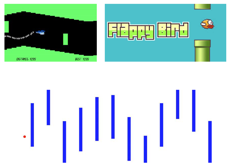
Suppose we have a drone which we want to fly avoiding obstacles, how can we model and compute the optimal trajectory?
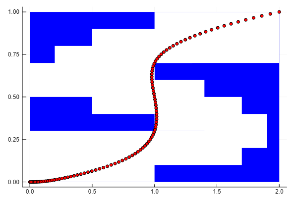
Let $(x(t),y(t))_{t \in [0,1]}$ represent the position at each time $t \in [0,1]$.
- Step 1: Discretize time intro intervals $0 = T_1 < T_2 < \dotso < T_N = 1$ and then describe position by polynomials $\{ p_i : [T_i, T_{i+1}] - > \mathbb{R}^2\}_{i=1}^{N}$ such that:
$$(x(t), y(t)) = p_i(t) \quad t \in [T_i,T_{i+1}] $$
-
Step 2: “Safe polyhedrons” $P^r = \{ x \in \mathbb{R}^2 : A^r x \le b^r\}$ such that: $$ \forall i, \exists r \text{ s.t } p_i(t) \in P^r \quad t \in [T_i, T_{i+1}] $$
- $p_i(t) \in P^r \implies q_{i,r}(t) \ge 0 \quad \forall t$
- Sum-of-Squares (SOS): $$ q_{i,r}(t) = \sum_{j}r_j^2 \text{ where } r_j(t) \text{ is a polynomial function}$$
- Boyund degree of polynomials:
SDP.
Using JuMP.jl, PolyJuMP.jl, SumOfSquares.jl, MI-SDP Solver Pajarito.jl for a 9 region, 8 time steps problem, we get optimal “smoothness” in 651 seconds as shown in the picture above.
While for 60 horizontal segments & obstacle every 5: Optimal “clicks” in 80 seconds.
Continuous solver?
- The
Hypatia.jlsolver: conic interior point algorithms and interfaces (Chris Coey, MIT)- A homogeneous interior-point solver for non - symmetric cones
- Versatility & performance = More Cones
- Two dozen predefined standard and exotic cones: e.g SDP, Sum-of-Squares and “Matrix” Sum-of-Squares for convexity/shape constraints.
- Customizable: “Bring your own barrier” = " Bring your own cone"
- Take advantage of Natural formulations.
- Take advantage of Julia: multi-precision arithmetic, abstract linear operators, etc.
- Modeling with new and nonsymmetric cones (Lea Kapelevich, MIT)
Tulip.jl: An interior-point LP solver with abstract linear algebra (Mathieu Tanneau, Polytechnique Montréal)- Set Programming with JuMP (Benoît Legat, UC Louvain)
- JuliaMoments (Tillmann Weisser, Los Alamos National Laboratory) -Dual of Sum-of-Squares
Daniel Pereda
Data Scientist
My research interests include optimization, game theory and operation research.